Fix point arithmetic vs floating point

See also discussion in https://www.microchip.com/forums/m487270.aspx

The advantage of floating point is obviously: There is no necessity to think about scaling, all multiplications runs well, scale from integer to float (measurement values), calculate in float, scale to integer for the actuator, ready, a simple obvious and manageable software.

Using fix point the scaling should not be a problem. Adding of different scaled values should not be a problem, but an manual programmed adaption of the scaling is necessary (which is done automatically by floating point addition). But each multiplying is a problem. Multiplying of two 16 bit values needs a 32 bit result, and then re-scale.

Using 16 x 16 ⇒ 32 bit multiplication in assembler using the best machine instructions is simple. But this is not supported by C/++. C/++ does not proper support such problems, as also not a fix point overflow. The programmer of this algorithm should know the machine instructions by thinking in C/++ statements.

If a processor contains a floating point hardware arithmetic, it is optimized. For example a cosf() (float cosinus) needs only 50 ns on a TMS320F28379D processor (and for this family) with 200 MHz clock. In opposite the fix point cosinus variant with interpolation second order (quadratic) with 14 bit accuracy (it is enough) need 400 ns. Because: It needs about 40 machine instructions. The cosf in float is built-in in the hardware and hence fast in about 10 clock cycles. If the interpolation will be supported also in the hardware, it may be fast. But unfortunately it isn’t so.

But, only comparison of single operations (cosf - 50 ns vs. cos16_emC - 400 ns) is not the real truth. Not a standard, but a specific algorithm is always assembled with machine code statements. Though a cosf is faster in float arithmetic as in int16, the whole algorithm may need more time in floating arithmetic. But this depends from the machine instruction, memory access possibilities (32 bit float number versus 16 bit integer), register architecture of the processor, and some other things.

Of course, if a floating point hardware artithmetic is not present, but fix point multiplication, the fix point arithmetic is more fast. This is true for some cheap and power reduces processors. Often a fast assembler-written floating point library is available. It means floating point operation does not need a long time. It is tested for the TLE9879 Infineon processor with 40 MHz clock: 1.5 µs for a cos16_emC(…​) 16 bit fix point operation, and 4 µs for the adequate cosf(..) float operations. It means using fix point is a quest of detail. If fast cycle times are necessary also in this actuator controller, it fix pint ay be necessary but also sufficient.

Some processors don’t have fix point multiplication, for example the MSP430 from Texas Instruments. Such processors are anyway not proper for fast step times (µs). They have libraries for fix point multiplication as well as floating point operations written in assembler. For such processors it is a quest of available memory (Flash and RAM) for a decision between fix and float numeric. The libraries need space in memory.

It is purposeful to use a value of 30000 to map the 1.0. Then an overdrive to 1.09 is possible. It is not purposeful to define the range of the int16 exactly from -1..+1, because the -1 is mapped to -32768 (-0x8000), but the +1.0 cannot be mapped, at least 32767. The fix point range is not symmetrically.

In a PLC ("Programmed Logic Control") such as Simatic S7 a nomial value of 27648 is used, see for example http://www.infoplc.net/files/descargas/siemens/infoPLC_net_Siemenes_S7_300_Escalado_Analogicas.pdf. There are many hits on a search engine in internet. This value is.

0x6c00 = 27648 = 3³*2¹⁰ = 3 * 3 * 2¹⁰ = 27 * 1024

This value is able to divide by 12 which may sometimes a good property. It has a possible overdrive till 118% or ~1.18.

Another proper value with possibility to dived is 27720. It is near to the PLC standard value, also with possible overdrive to ~1.18, but it is able to divide by more numbers:

0x6c48 = 27720 = 2 * 2 * 2 * 3 * 3 * 5 * 7 * 11

able to divide by 2,3,5,6,7,8,9,10,11,12,14,15,16,18,20,22,24 ,28,30,32,33,35,36,40,42,44,45,50,60

The number 25200 as nominal value for 16 bit integer allows an overdrive till 130% or 1.3 which is usual enough for technical systems. It is able to divide by 100, 90, 80, 75, 70, 60, 50, 45, 40, 35, 30, 28, 25, 24, 21, 20, 18, 16, 15, 14, 12, 10, 9, 8, 7, 6, 5, 4, 3, 2 without fractional part.

0x6270 = 25200 = 2 * 2 * 2 * 2 * 3 * 3 * 5 * 5 * 7

This numer should be the best for scaling 16 bit fix point numbers with a nominal value of 1.0 and overdrive till 130% or 1.3, a resolution of near exactly 0.004%, which can be divided by the most of important factors. It is a universal number and also imageable while debugging.

Hence this number is defined in emC/Base/Math_emC.h as

The number 23170 = 0x5A82 is approximately sqrt(2)*0x4000 (exactly 23170.4750). If a value is normalized with this, the quadrat of the value is normalized to 0x4000 and can be used for further calculation of a magnitued (see #sqrt and #rsqrt). An overdrive till 140% is possible. It is defined as

But because often multiplication and bit shifting is important, the scaling should be oriented to 0x4000, which allows overdrive to 1.999 and its resolution is enough with 1/16385, better than 0.1 promille.

It should be proper to use the same number as nominal value as for int16, but only expanded to 32 bit. This is

1651507200 = 0x62700000 = (25200)<<16 = 2²⁰ * 3 * 3 * 5 * 5 * 7

The Overdrive is about 130%, the resolution is enough fine.

The other variant is, scaling to 0x40000000 for 1.0.

The nominal values in the chapters above are proper able to use for add and sub operations. The nominal range is not changed while this operations are done.

But the multiplication does not work proper. For multiplication another thinking is necessary:

If 1.0 is scaled by 25200 as int16, the multiplication of 1.0 * 1.0 should also result in 1.0, it means 25200 in this scaling. But this is not so.

For factors, a scaling exactly as 2ⁿ is necessary. After multiplication the result should be shifted. See example:

One can test it with a normal hexa calculator on PC. It is a simple unsigned integer multiplication. But see next chapter.

If you multiply a nominal scaled value with a factor which is guaranteed <1.0, you can set the decimal point left side of all bits. 0xffff then is mapped to 0.99998. 0x8000 is exactly mapped to 0.5. Then you can multiply without additional shifting. The result is proper in the same scaling but with double bit width:

If you use only the upper 16 bit as result, you get 0x626f = 25199 which can be scaled to 0.99998 if the NOM1_i16_Ctrl_emC = 0x6270 scaling is used.

You should never have the idea to scale a factor with one of the nominal values not as power of 2. Why not? For example you have a factor which may be > 1.0 but never > 1.18. Then you may use the nominal value 27648 as proposed in Simatic S7, have a value of 1.05, convert it to 29030 = (int16)(27648 * 1.05f), multiply for example with 1.0 =^ 27648, and get 802621440 = 0x2FD70800. But what’s that for a number? You should multiply it with the reciproke by scaling to get the scaled value already. It is a non constructive effort.

For that example you should scale your factor as fractional part of 2ⁿ as 0x8000 =^ 1.0. It is seen as unsigned uint16. Then multiply using NOM1_i16_Ctrl_emC for only (!) the first factor:

You can use only the high part (to save effort), and shift it to left by 1 bit.

Test:

This is the proper result in the same scaling as the input value. The possible exact result 0x675C was not calculate because of rounding effects.

Rule: You can use a special scaling for one of the factor, the physical value, but you should always use a power-of-2 mapping of the second factor.

A multiplication can be done inside the processor as 16*16 bit result in 32 bit, as 32 * 32 bit result in 64 bit. The result is without overflow. You can select the proper part and shift to get either back to 16 bit or back to 32 bit, but it is possible to produce an errorneous value if the range of the result is violated. You should know your value range. You should avoid elaborately range tests, it needs more calculation time as using the higher bit resolution.

Often, especially for integrators it is recommended to use the 32 bit width for 16 bit input values for further calculation. The end result can be shorten then, for the output value.

It is very simple. An angle between 0° and 360°, or better between -180° .. 0° .. 179.9999° can be represented with the full integer range:

There is a very important advantage: The angle is full defined in a 360° circle. The difference (-181° - 179°) is as expected simple 2°. It is because integer arithmetic has no overflow handling. The values are closed between 0x7fff..0x8000. For example if a T1-FBlock (smoothing block) is necessary and the angle varies in range around 180°, no problem. For float representation it is a concise problem: Always overflow > PI and < -PI should be handled.

Hence it is better to use this angle representation also for floating point environments, with a simple conversion:

Calculation angle values, especially differences should be done using integer arithmetic. Before using the angle value as float, the simple multiplication above should be done.

In emC/Base/Math_emC.h there are defined some macros which can be adapted to proper assembly instructions, especially for ARM, for this saturating operations. The standard implementation is defined in C language, proper but not full optimized for all processors.

The signed subtraction can anyway performed by using the negated value with signed add, though the ARM has also a signed saturation subtract.

Some more instructions, sometimes necessary, regard some especially assembly instructions of the ARM, maybe similar also in other processors:

This instructions which handles two operation with one assembly instruction may be necessary especially for 16 bit integer operations. The 8 bit saturation operations are not (yet) supported by macros. This operations are familiar for color calculations, not the focus of embedded algorithm. They can be created if necessary.

This macros are defined in C language in a common proper way in emC/Base/Math_emC.h. For a specific processor this macros can be defined especially using the __asm(…​) definition in the compl_adaption.h. Because of #ifdef adds16Sat_emC etc. is tested, this specific definitions of the macros in compl_adaption.h are used.

Using this macros enables optimized usage of machine instructions though it is programmed in C/++.

On ARM processor the saturation operations set the Q flag if a saturation occurs, and let it unchanged elsewhere. The usage of this should due to the following pattern:

On saturation a warning or such can be noted. The saturated result is able to use, this is the approach of saturating arithmetic. Evaluating the Q flag is only for additional information.

But this additional information may be necessary. Hence the macros for saturation arithmetic in C language regard this too.

It is necessary to write the following macro in a statement block which uses the saturating macros:

To check whether saturation has occured, it can be tested:

The usage of this flags are optional, if necessary. If this macros are not used, the effort for the boolean variable in DEFsatCheck_emC is removed by optimizing compilation.

If this macros are adapted to a specific machine set (in compl_adaption.h), for the ARM processor it should check and clear the Q flag.

There are also some "add and multiply" instructions, and some instructions to detect overflow. Reading some manuals of processors, it seems to be adequate to program such parts in assembler. The link: https://www.quora.com/How-much-could-we-optimize-a-program-by-writing-it-in-assembly discuss some of good or bad reason to program in assembler, see there the contribution from Hanno Behrens: "Do people still write assembly language?".

From position of producers of tool or processor support, it is appropriate to deliver some libraries for expensive mathematical and control algorithm (including PID-control with some precaution of integral windup and such things). The application programmer can use it, no necessary for own mathematics. But this approach obliges a user to the one time selected hardware platform. The programs are not portable. There is no standard (for C/++) to unify such libraries.

The C/++ language allows constructs to implement specific assembly instructions. That is an advantage of C language. In this kind specific macros or inline functions can be defined as interface, which can be simple implement by inline-assembly statements or macros with specific castings (one time written) for any processor, respectively a standard implementation with C-code exists, which may be enough fast for first usage.

The emC concept is predestinated to support such ones, because it is "embedded multi platform C/++". Hence it do so.

The following operations (may be specifically implement as macro or inline in the compl_adaption.h) are defined and pre-implemented in C (emC/Base/types_def_common.h):

Additional there are some more instructions which supports the "mult and add" approach.

This operations cannot be a part of an expression, they are in form of statements. For that it is sometime more simple to build proper macros or assembly expressions.

Why a signed or unsigned distinction is not necessary for the mul32lo_emC? Because:

The lo part of a multiplication is the same independent of the sign of the inputs.

This is adequately similar also for a mul*16_emC. The essential thing is: The inputs should be exactly enhanced to its 32 bit form, then multiplicate 32 * 32 bit, and use the lower result. But: That is more effort. The multiplication 16*16 bit to 32 bit needs lesser time and hardware resources. Only the sign should be automatically correct expanded.

That’s why usual embedded processors have often machine instructions for multiplications:

That are the same as the mul*_emC instructions above. That are the usual necessary ones.

A multiplication operation 32 * 32 bit to 32 bit lower part is often offered as machine code instruction.

Generally the 32*32 bit multiplication using the lower 32 bit result may have an overflow problem. Then the result is not useable. But:

If the sum of the relevant input bits does not exceed 32, then the result is correct.

In contrast to the 16*16 bit multiplication, it is possible for example to use 24 bit resolution of a signed number for one factor, multiplied with a factor which needs only 8 bit. That can be a gain from 0..15 with resolution 1/16 or for the user: 0.1. It is fine enough for some applications. The gain is scaled 1.0 =^ 0x10. Example multiply -1.5 * 1.0667, the scaling of the first factor is 1.0 ^= 0x00'400000, which allows a 24-bit-range -2 .. +1.999, but before multiplication a limitation may be done to prevent overflow. -1.5 ^= 0xFF’A00000

It is important that the both 32 bit factors are exactly expanded with the sign. It means the 24 bit value 0xA00000 (negative) is expanded to 0xffA00000 and the 0x11 (positive) is expanded to 0x00000011. The result is correct if the sign of the factors are correctly expanded. A difference between signed and unsigned multiplication is not done.

The resulting value is 0xF9A00000, the higher part 0x00000010 of the theoretical 64 bit result is not built. The result should be shifted 4 bit to right because the second factor has 4 dual digits in the fractional part:

This is near the input value, only multiplied with 1.0666, presenting

Note: The negative 24 bit number 0x9a0000 is 0x660000 negated, usual 32 bit arithmetic is used, -0xff9A0000 ⇒ 0x00660000.

If you want to multiply 16 * 16 bit signed or unsigned to 32 bit, you should expand the input values exactly like necessary for the sign, and simple multiply. To better understand, the numbers have its decimal point after 4 bits, the input range is -8.0 .. -7.9999. The decimal point of the result is with 8 bits before.

In C it is:

That are the standard definitions of the both macros. The usage is:

That delivers anyway the correct results. The compiler may recognize that the inputs have only 16 bit because of the mask and type casting. It is able to expect that the compiler uses its best machine code which may be a 16 * 16 ⇒ 32 bit multiplication.

It may be possible, depending on the compiler properties, that the following term is sufficient:

But that is not sure in any case. Hence this writing style is not portable. See also

https://www.ti.com/lit/an/spra683/spra683.pdf.

It may be possible that the result has 16 bit and it is expanded to 32 bit, or it works exact. Unfortunately the C standard does nothing guarantee.

For some compiler an __asm(…​) statement can be used to select the desired machine code. This can be written as:

This is an example for ARM processors. The ARM M3 has the 32 * 32 ⇒ 32 lo-bit multiplication, see chapter above, but not dedicated 16 * 16 ⇒ 32 bit multiplication machine statements because the ARM machine has always 32 bit width. The MUL instruction works with two registers, one operand should be the same as the destination. Hence there is no possibility for a optimization. The compiler produces similar results on using the standard macros.

It depends of the type of processor. The Texas Instruments TMS320C2xx processor has the 16 * 16 ⇒ 32 bit MPY statement, but the C2000 compiler does not support __asm(…​) instructions with self defined register, it supports only simple static machine code. But the compiler is optimzing too without the asm macros.

For writing the __asm macro for gcc compiling, and also for ARM compiling (AC6) see:

https://gcc.gnu.org/onlinedocs/gcc/Extended-Asm.html

The data are defined in emC/Ctrl/T1_Ctrl_emC.h as:

The 32 bit values are also accessible as 16 bit parts by building a unit. Therefore a struct Endianess32_16_emC_s is used which contains only a unit to access the 32-bit- and the 16-bit hi and lo parts. This struct is defined depending on the endianness of the processor.

The T1-factor is built with:

To convert the factor, floating point arithmetic is used. In a cheep 16 bit processor it is calculated by software, needs a longer time but the factors are usual calculated only in startup time or in a longer cycle. It is possible to give factors also without conversion, or via conversion over a table, to speed up it. The factor has the decimal point left, and up to 32 fractional bits.

The calculation usual called in a fast cycle is simple. It uses a 16 * 16 ⇒ 32 bit multiplication, which is fastly usual available also in cheep processors. The 32 bit result is used for the integration. The result value uses the higher 16 bit part of this integrator.

The possible higher accuracy of (x - thiz→q) is not used in this algorithm. But this may be necessary for longer smoothing times. The algorithm above limits the smoothing time to about 65000 * Tstep, because the used high part of fTs is then 0x0001, for greater times it is 0x0000 and nothing occurs.

If it is necessary to use longer smoothing times, it requires a 32 * 32 ⇒ 32 bit multiplication, where the higher part of the 64-bit-result is used. A further improvement may be possible to use a 64-bit-width integrator, but this is not realized here. It is a quest of calculation time effort. The better step routine for longer smoothing times can be called in the application:

Right shift (…​)>>32 takes the one 32 bit result register from the multiplication, ignores the lower multiplication result. But that is true for this algorithm. Right shift (…​)>>32 takes the one 32 bit result register from the multiplication, ignores the lower multiplication result. But that is true for this algorithm.

The dx part can be used as differtiator with smoothing, simple accessible after this calculation with

The outside used values are all 16 bit, for a 16 bit controlling algorithm on a 16 bit controller. But the internal state of the smoothing block is stored as 32 bit. Both, it results in the machine execution of the multiplication, and (!) for the resolution of the smoothing. You can use a great smoothing time, and get exactly results without hanging effect.

If floating point arithmetic is used, the algorithm is more simple to write and understand, but you get the hanging effect for lesser smoothing time (disadvantage of the implementation) and you need always more calculation time, also if a floating point calculation hardware is present.

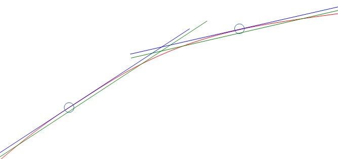
The red curve should show the really function.

The blue lines are the tangents. Near the point itself the linear approximation is accurate as possible. But between the points a greater abbreviation is given. This can be redeemed by a second order (quadratic) approximation, not shown here. As tested the quadratic approximation delivers errors less or equal 4 for 16 bit numbers, with only 16 supporting points, a well useable result.

dx := (x - x_p);

y := y_p(x_p) + g_p(x_p) * dx + g2_p(x_p) * dx²;

Where g_p is the tangent (the exactly deviation of the curve) or the quotient

g_p = (y_p+1 - y_p-1) / (x_p+1 - x_p-1);

and g2_p is the difference of the g_p of the left and the right point:

g2_p = ( (y_p+1 - y_p) / (x_p+1 - x_p) ) - ( (y_p - y_p-1) / (x_p - x_p-1) );

If the step width between the points in x are equidistant: x_pp, it is more simple:

g_p = (y_p+1 - y_p-1) / ( 2*x_pp);

g2_p = ( (y_p+1 - y_p) - (y_p - y_p-1) ) / x_pp;

This is the same as shown for example in https://www.astro.uni-jena.de/Teaching/Praktikum/pra2002/node288.html, (visited on 2021-04-13), only the term for the quadratic part is shown there more 'mathematically', but it is the same: `( (y_p+1 - y_p) - (y_p - y_p-1) ) == (y_p+1 - 2 * y_p + y_p-1). The left form prevents overflow in calculation with fix point arithmetic.

Simple linear approximation but with middle-correct of abbreviation

But the algorithm for a linear approximation is very simple:

y := y_p(x_p) + g_p(x_p) * (x - x_p)

x_p is the x value where the nearest point is found. g_p and y_p are read from the table. dx = x - x_p is left and rigth side from the point.

The green lines are slightly shifted. The error on the supporting points are approximately equal to the error in the middle, the error is halved. But this is not the most important effect. More important may be that an integration does not sum up the deviations only in one direction. It can be seen on cos values: Its integration should deliver sin values, and the area or the range -Pi .. Pi should be 0. The calculation is the same, but the values are corrected in the table.

For the C/++ implementation the tables contains valued immediately given as hexa values. But this values are calculated by a Java program, using the double precision functions, with the named correctures. See org.vishia.math.test.CreateTables_fix16Operations (https://github.com/JzHartmut/testJava_vishiaBase).

In C language the core algorithm for the linear approximation is written as (emC/Base/Math_emC.c):

It is a macro used in some functions, see below. The expanded macro is well for compilation. Using an inline function may have disadvantages, for example calculation (16 - BITSEGM) as compiler constant. This macro is defined only in the compiling unit emC/base/Math_emC.c locally, not common useable.

valTable: For faster access on 32 bit processors only one value with 32 bit is read from the table. The high part is the supporting point, the low part is the gain. The gain is dispersed in the next line.

Index to the table: The x value in range 0x0000 .. 0xffff supplies the index to the supporting points. Depending on the size of a segment, given in BITSEGM as number of bits, the x value is shifted to right. Adding (1 <<(BITSEGM-1) before shifting gets the index of the right point for the right part of a segment. The index calculation are a few operation in a 16 bit register. The value (1 <<(BITSEGM-1) is calculated as constant by the compiler anytime. Example: BITSEGM = 9 means, a segment is for example from 0x3c00 .. 0x3e00, 9 bits. For a value 0x3d65 a 0x100 is added (1 << 8), and after right shift from 0x3e45 the value 0x1f as index to the table results.

dx: The difference value inside the segment is taken from the x value shifting to left, shift out the index bits. The dx is positive or negative. Example: For the value 0x3d65 a shift to right with (16-9 ⇒ 7) bits is done and results in 0xB280. The operation & 0xffff is optimized because the compiler may or should be detected that it is only a 16 bit operation. Visual Studio may detect a run time error because it expands the numeric range to int32 and checks the follwing casting, if & 0xffff was not written there, though x is an int16 and the operation should be performed as int16 operation. Java does similar, but for Java it is defined in the standard, that all integer operations are executed with at least 32 bit.

muls16add32: The multiplication uses both 16 bit values. The useable result is located only in the high bits 31..16 of the multiplication result. Hence the addition with the whole table value with the supporting point in bit 31..16 would add correctly 16 bit with round-down if the lo bits 15..0 of valTable would be set to 0. The Savings of this operation gives a possible overflow, an error of only one bit. This is not relevant, calculation time saving is more relevant.

int y: The operation (int16)(valTable >>16) uses 32-bit half register operations or uses the 16-bit-register immediately. As expected all compiler detects this situation, and do not produce the >>16 operation, except it is a 32 bit processor without access to half register.

Adequate the (int16)(valTable & 0xffff) is a optimized half-register optimization, without mask with 0xffff which would need loading a constant in machine code.

Hence this operation is so fast as possible.

sin and cos are adequate, only shifted by 90°. Hence the cos is programmed, and the sin is derived with:

The cos is symmetric on y-axes and point-symmetric for 90°. The interpolation need only be executed between 0° and 90°:

Because the reduced x range only 32 and not 128 supporting points are need. This reduces Flash memory amount. But the preparation increases the calculation time. Hence it may be dismissed.

More simple is, using 64 supporting points and only build the absolute value. Results from positive and negative angles are exactly the same.

This is the whole cos16_emC operation, with all comments for experience (2021-04-07).

The cosTable looks like (shortened):

The value for 0° is set to 0x7fff which is 0.99997, because the value of 1.0 cannot presented. 90° is exactly 0, and 180° (angle 0x8000) is exactly 0x8000, which is -1.0. The error of approximation is at max -8..8, tested. It is greater in the ranges around 0° and 180°, lesser near -1..1 in the range around 90°. Using the sinus with the same operation (only the angle is shifted) means, a sin in the linear range around 0° has only an interpolation error from -1..1 related to 32768.

The Java algorithm to get the supporting points and gain uses double algorithm and rounding. It is written commonly for any mathematic function. See snapshot of org.vishia.math.test.CreateTables_fix16Operations.java:

Firstly an internal interface is defined for all the functions.

The common operation to create a table is:

It is a common operation for all mathematic functions to support tables. Invocation for the cos is:

There are some manual given points, especially 0x7fff and 0x8000 for the first and last point. Elsewhere the algorith calculates a value of 0x7ffc and a gain of 0 for the first segment. The point {32, 0x0} is the value for 90°, which should exactly much. But the value is calculated to 0 also without this setting because the cos is linear and point symmetric in this range.

The segment size is 9 bit =^ 0x200. With 64 values the range 0x0..0x8000 is produces. The Math.PI is the x scaling for this range. 1.0 is the y scaling regarded to 0x8000.

The expression (x)→ Math.cos(x) is a "Lambda expression" in Java, a simple kind to provide a function.

"cos" is the name of the table "cosTable". This routine generates all points, test all points with printf-output for manual view and writes the file yet to T:/<name>Table.c.

Java is a more simple programming language and hence proper for algorithm tested on PC, as preparation for embedded software. Same written and tested in C++ is more complicated. It is not necessary. The advantage of Java is: It has the same approaches for integer processing as C/++.

An important function to get the angle from a complex presentation is the arctan2 operation. Normally it divides both values and uses either the arctan or the arccot operation.

This is the proven concept, uses stable mapping of mathematic functions and prevent division by zero. But: It needs a division which is not a cheep operation for fix point arithmetic.

There is another way to calculate:

Usual either the values for the { re, im } vector are normalized or the magnitude is a point of interest, and the normalization is a more cheap and by the way occurring operation.

Hence the arctan is defined for normalized values and uses a arccos table. The arccos does not need a decision, it is a continuous table.

This is the whole algorithm, see emC/Base/Math_emC.c. Simple comparisons determine one of the 8 segments of the result. The input for the linear interpolation is always in range 0x0000 .. ~ 0x2d80 which is a proper range for the approximation.

The normalization of the x-input is 0x4000 for 1.0. Hence the lesser value of re and im part is never greater then ~sqrt(2)*0x4000 which is approximately 0x2d41. But less errors for the normalization may force a slightly higher value. But the asinTable goes to 0x4000.

The calculation time of this solution for 16 bit fix point is approximately the same as a floating point atan2f(im, re) operation of the math.h standard library for C, measured on the TMS320F28379 Processor from Texas Instruments, which has Floating point support. In opposite most int16 or int32 operations needs about 150% of the calculation time compared with the floating point calculations on that processor,

How to normalize:

The normalization is often anyway necessary. To get the magnitude (not only the revers magnitude) either a division can be used, or it is gotten also with the Nom_int16_complex.

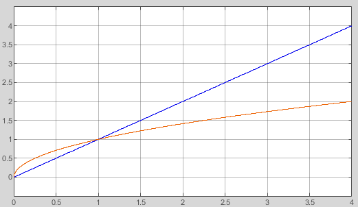The square root is only defined for positive numbers. Hence the input range can be from 0…​ <4.0 mapped to 0x0 …​ 0xffff. The sqrt is then in range 0..<2.0 which can be mapped to 0x0…​0x7fff. The result can be used than as signed value.

is defined in that kind. The value 0x4000, mapped to 1.0, results in 0x4000.

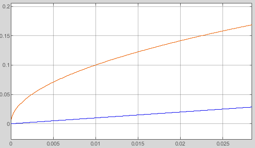The sqrt function has a problem in 0-range. The deviation of sqrt is 1 / (2 * sqrt(x)). This is infinitive for exact 0. The right image may show that the sqrt line (red) is perpendicular at the point 0. If the linear approximation is used with equal distances in x, it has a problem in the first segment. The linear connection does not represent useable values.

But: Is an exact sqrt necessary for values near 0? Often values in the nominal range are the point of interest. It means between 0.5 …​ 2 of the nominal values. In that range the simple linear approximation of the sqrt is well useable. The test of results of the sqrt16_emC(…​) uses values started from 0x600 only, it is ~ 0.1. From this value the abbreviation is <9, it is <0.1% regarded to the value 0x4000 =^ 1.0.

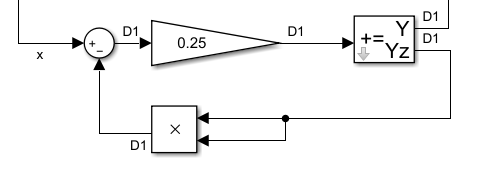To get the sqrt in controlling systems there is another possibility shown in the right image. The x-value (the quadrat) is delivered as the input of a controller feedback. The feedback is the output multiplied with itself. This is compared with the input, and the controller will control it to the equal value (zero-deviation). Hence the output of the controller is the sqrt because the feedback is the square. See also chapter #Nom_int16_complex

This can be used anytime if the input value x does not change in a wide range for one to the next step, as given in usual controlling systems. But also for the step response of the control loop only a first deviation is given. It is fast.

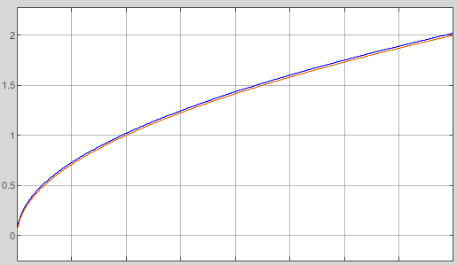The gain of this controller loop should depend on the max possible value of the output, with multiplication the gain in loop should be < 1.0. This is true for the right image for input values less than 4.0.

The right image shows the controller output and the calculated sqrt. Both curves lie on top of each other. An additional offset of 0.02 is only used to see both curves in the diagram.

The reciprocal or inverse square root can be used to normalize a value. The value should be multiplied with the reciprocal square root of the quadratic sum of the components:

rm := rsqrt(y.re * y.re + y.im * y.im);

y_nom(re, im) := y(re, im) * rm;

The magnitude itself is not calculated with this, but the division, more expensive for simple controller, is prevented.

m := sqrt(y.re * y.re + y.im * y.im);

y_nom(re, im) := y(re, im) / m;

…​needs two divisions, for real and imagine part, instead two more cheap multiplications.

But, the value for 0 is infinitive. It is mapped to the max possible value, it is 0x7fff =^ 1.9993. Lesser values than 0x14a0 =^ 0.322 deliver a result which is lesser as expected. It means using for normalization delivers to less values. The supporting point table has 33 entries. Values from 0x14a0 = 0.322 till 0x27a0 =^ 0.641 may have an abbreviation till 42/16384. Values from 0.641 .. 1.9993 may have an abbreviation ⇐10 / 16384 which is < 0.1%. It means for values near the nominal value 1.0 =^ 0x4000 it is proper useable.

works in range 0 …​ 1.9993 mapped as 0x0 .. 0x7fff and delivers a value in range 1.9993 …​ 0.5 mapped to 0x7fff .. 0x2000 as int16 result.

If the sqrt16_emC() is used for normalization or for any other reason the reciprocal value may need:

y := 1 / x;

Because a division is a non-cheap operation on some controller without specific division hardware support, using a linear approximation is also possible and evident to use.

This is a class for a controlling algorithm to get the nominal values of a vector and/or the magnitude.